Hearing in marine fauna
Marine animals rely heavily on sound for all major life functions as the acoustic energy propagates in water more efficiently than almost any other form of energy. For example, mammals and fishes produce sound during communication, reproduction, nursing, navigating and foraging. They use sound to coordinate group hunting and mating. They passively listen to the environment for navigation. They actively echolocate (toothed whales) on prey and passively listen to prey. With the deep ocean being devoid of light, animals rely on sound for survival.
Since the onset of the industrial revolution, the oceans have become increasingly noisy. Noise from ships, offshore oil and gas exploration, near-shore construction, deep-sea mining, naval exercises, etc. fills the oceans and, in places, can be heard hundreds of kilometres away because sound propagates so well underwater. The volume and spatial extent of marine noise pollution have become one of the significant threats to animals and their habitats. Noise has the potential to interfere with animal acoustic communication and sensing. Noise has been linked to at least one incidence of cetacean mass stranding. Predator-prey relationships may become unbalanced. Energetic costs of animals may rise as they change behaviour, location or acoustic signalling in noise. Stress levels have been shown to increase in the presence of underwater noise. In extreme cases, close to the source, high-intensity noise can injure animals by causing acoustic tissue trauma.
Previous studies have shown the impacts of some types of noise on selected animal species, however, the effects of a variety of noises on the vast majority of animals are unknown. There are many missing links due to most of the species being unavailable in aquaria or laboratories for live, traditional, experimental work. For instance, we lack information on the cumulative effects of repeated exposure to the same or different types of noise over the course of a season or migration cycle. More importantly, we lack a fundamental understanding of what the vast majority of marine animals can hear making it impossible to assess the effects of noise. This research stream can overcome these challenges and fill some of the missing links. The aim of this work is to develop fast, reliable, non-invasive and efficient techniques that construct acoustic propagation and reception models based on high-resolution biomedical imaging of collected naturally deceased animals. The numerical models are used to study internal sound propagation and reception pathways, as well as the interaction of the noise signals with various structures in the animal head and surrounding media. With this work, a database of hearing and noise impacts in marine megafauna will be developed to provide fundamental information on hearing and hearing impairment to animals to empower managers of ocean ecosystems.
Our research combines numerical techniques (Finite Element Analysis-FEA) with CT/MRI imaging data and anatomical measurements to simulate the sound propagation and reception pathways through complex biological structures and surrounding media.
CT/MRI scan and data analysis
CT/MRI imaging is a non-invasive technique, and can provide very detailed information on animal structures without causing any damage to the specimen and can be used for constructing accurate numerical models.
We collect fresh stranded specimens for high-resolution CT/MRI scanning. For the large-sized whales, only the ear parts are scanned, for the middle-sized dolphins and whales, only the heads of the specimens are scanned, and for the small-sized animals, such as fishes, the whole body is scanned.
We extract geometry information of the specimens and export the Hounsfield Unit (HU) values of tissues for three-dimensional (3D) model construction. Figure 1 shows an example of a CT scan of a bottlenose dolphin.

Anatomical measurement
We slice the specimens for the tissue property measurements, as shown in Figure 2.

For the sound velocity measurement, an ultrasonic pulse-receiver with MHz centre frequency is used to emit the signal through each sample. The signals reflected from two boundaries of the samples are recorded to obtain the time difference (t). The distance between the two boundaries (d) is measured using a vernier calliper. Then the sound velocity (c) of each tissue can be determined (c=2d/t). For the density measurement, we use a high accuracy electronic balance to measure tissue mass (m). The volume of samples (V) is measured as the amount of water displaced using a high accuracy cylinder. The density of tissue can thus be determined (ρ=m/V).
3D Acoustic property reconstruction
Based on the measurement results, we derive the acoustic impedance of each tissue sample by function Z=ρc. The relationships of HU-to-sound velocity, HU-to-density and HU-to-acoustic impedance are determined by regression analysis. We then convert the CT information into acoustic impedance models of the specimen for simulation.

Numerical modelling
FEA is a numerical technique for finding approximate solutions to boundary value problems for partial differential equations. The advantage of the FEA is the ability to deal with the complex boundaries and to provide fine spatial information of the animal heads. We import the impedance models of the specimen and overlay with the fine mesh with acoustic impedance values at the nodes. A mesh refinement analysis is performed to find the optimal element size for each model. The inhomogeneous wave equation is solved with the FEA at each grid:
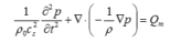
where denotes the equilibrium density (kg/m3),
 is the speed of sound (m/s), and
 is a monopole source, respectively. Figure 4 shows an example of a FE model construction process based on CT scan data.

The non-invasive and fast methods we have developed allow us to study internal sound propagation and reception through biological structures. The models can determine what frequencies these animals can hear and can predict the hearing range of some species of animals, as well as assess the risk of noise damage to animal hearing.
